In probability theory and statistics, the multivariate normal distribution (MVN) is a generalization of the one-dimensional normal distribution to higher dimensions. This article will explore the concept of MVN, its properties, and several tests for assessing multivariate normality.

Properties of MVN

The MVN is characterized by a mean vector $\mu$ and a covariance matrix $\Sigma$. The joint probability density function (PDF) of an MVN is given by:

$$f(\mathbf{x} | \mu, \Sigma) = \frac{1}{\sqrt{(2\pi)^n |\Sigma|}} \exp\left(-\frac{1}{2} (\mathbf{x}-\mu)^T \Sigma^{-1} (\mathbf{x}-\mu)\right)$$

where $\mathbf{x}$ is a random vector, $n$ is the dimension of the space, and $|\Sigma|$ is the determinant of the covariance matrix.

Multivariate Normality Tests

Several tests have been proposed to assess whether a given dataset follows an MVN. Some of these tests include:

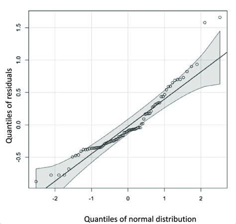
• Q-Q plot: A Q-Q plot (quantile-quantile plot) is a graphical method that plots the quantiles of two datasets against each other. In the context of multivariate normality, we can use a Q-Q plot to compare the distribution of our data with the expected MVN distribution.
• Mahalanobis distance: The Mahalanobis distance is a measure of the distance between a point and an MVN. This distance takes into account both the mean vector and the covariance matrix of the distribution.

Example Code in R

The following code demonstrates how to perform some of these tests using the mvtnorm package in R:

library(mvtnorm)

# Generate sample data
set.seed(123)
n <- 100
p <- 5
X <- rmvn(n, mean = c(0, 0, 0, 0, 0), sigma = matrix(c(1, 0.3, 0.2, 0.1, 0.05,
 0.3, 1, 0.4, 0.3, 0.15,
 0.2, 0.4, 1, 0.6, 0.25,
 0.1, 0.3, 0.6, 1, 0.35,
 0.05, 0.15, 0.25, 0.35, 1), nrow = p))

# Perform Q-Q plot
qqplot(X, main = "Q-Q Plot of MVN")

# Calculate Mahalanobis distance
dist <- mahal(X, mean = c(0, 0, 0, 0, 0), sigma = matrix(c(1, 0.3, 0.2, 0.1, 0.05,
 0.3, 1, 0.4, 0.3, 0.15,
 0.2, 0.4, 1, 0.6, 0.25,
 0.1, 0.3, 0.6, 1, 0.35,
 0.05, 0.15, 0.25, 0.35, 1), nrow = p))

# Plot Mahalanobis distance
plot(dist, type = "h", main = "Mahalanobis Distance")

Srivastava Test for Paired Multivariate Data

The Srivastava test is a statistical test that can be used to compare the mean vectors of two paired multivariate datasets. This test is implemented in the multifluo package in R.

Here's an example code snippet:

library(multifluo)

# Load sample data
data1 <- mechanics + vectors
data2 <- algebra + analysis

# Perform Srivastava test
sri.test(data1, data2)

This code performs the Srivastava test on the two paired multivariate datasets data1 and data2. The output will include a p-value, which can be used to determine whether the null hypothesis of no significant difference between the mean vectors is rejected.

In this article, we have explored the concept of multivariate normality, including its properties and several tests for assessing MVN. We have also provided example code in R using the mvtnorm and multifluo packages to demonstrate some of these concepts.