======================================================
Quantile-Quantile (Q-Q) plot is a graphical tool that helps us assess whether a set of data plausibly came from some theoretical distribution, such as Normal, exponential or Uniform. Additionally, it helps determine if two data sets come from populations with a common distribution.
Advantages
- Flexible: Q-Q plot can be used with sample sizes.
- Robust: Many distributional aspects like shifts in location, shifts in scale, changes in symmetry, and the presence of outliers can all be detected from this plot.
Scenarios Checked
- Common Distribution: Whether two data sets come from populations with a common distribution.
- Common Location and Scale: Whether two data sets have the same mean and standard deviation.
- Similar Distributional Shapes: Whether two data sets have similar distributional shapes (e.g., symmetric or skewed).
- Similar Tail Behavior: Whether two data sets have similar tail behavior (i.e., extreme values).
Interpretation
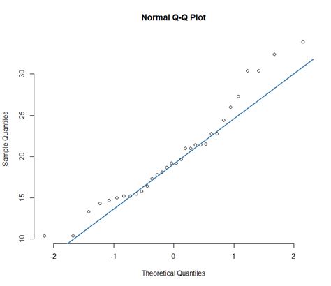
A Q-Q plot is a plot of the quantiles of the first data set against the quantiles of the second data set.
- Similar Distribution: If all points lie on or close to a straight line at an angle of 45 degrees from the x-axis.
- Different Distribution: If all points lie away from the straight line at an angle of 45 degrees from the x-axis.
Python
The statsmodels.api package provides qqplot() and qqplot_2samples() to plot Q-Q graphs for single and two different data sets, respectively.
Interpreting Shape of QQ Plot of Standardized Residuals
When interpreting the shape of a Q-Q plot of standardized residuals, we can identify several patterns:
- Fatter Tails: The ends of the line of points turn counter-clockwise relative to the middle, indicating that the tails of your distribution are fatter than those of a true Normal distribution.
- Mixture of Distributions: The shape suggests that you have a mixture of two distributions with the same mean but different standard deviations.
Code Example
The following R code can be used to generate a plot similar to yours:
set.seed(646) # this makes the example exactly reproducible
s = 4 # this is the ratio of SDs
x = c(rnorm(11600, mean=0, sd=1), # 99.7% of the data come from the 1st distribution
 rnorm( 400, mean=0, sd=s)) # small fraction comes from 2nd dist w/ greater SD
qqnorm(x) # a basic qq-plot
The Q-Q plot is a powerful tool for identifying and understanding the underlying distribution of your data. In this article, we have discussed how to interpret the Q-Q plot in linear regression and how to identify common scenarios such as different distributions, locations, scales, shapes, and tail behaviors. Additionally, we have shown an example code in R that can be used to generate a plot similar to yours.